Understanding the Muon Optimizer

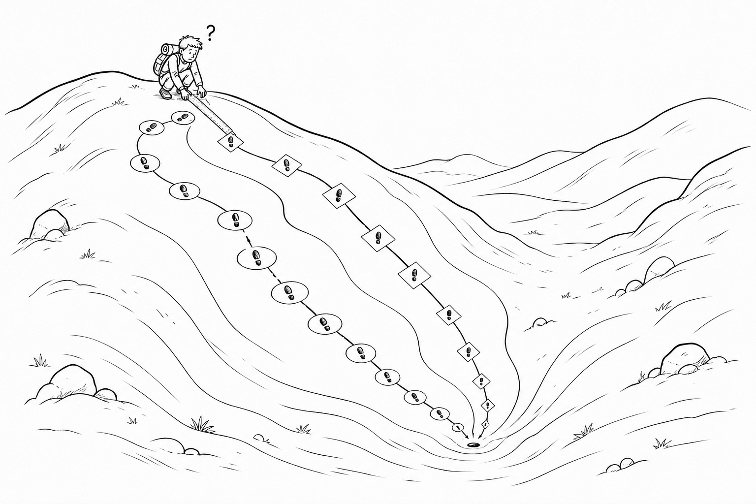
Before diving into Muon, I found it helpful to revisit the intuition of gradient descent. Imagine you find yourself in a landscape with hills and valleys, and you want to reach a low point in a valley. How should you choose a path to get there (there is more than one!)? Gradient descent tells you to step in the direction of the fastest local drop in altitude per unit of step length. There is an interesting detail hidden in that sentence: the direction of the fastest drop with respect to step length actually depends on the geometry you use to measure your step length! The most straightforward choice is the Euclidean metric, using the $L_2$ norm for vectors or the Frobenius norm for matrices. This gives the familiar negative-gradient direction.

Mathematically, the steepest descent direction under the Frobenius norm can be obtained by minimizing this linear approximation within a fixed step budget:

Here, $\eta$ is the step budget, $\Delta W$ is the change in a weight matrix of the neural net, and $\langle A,B\rangle=\operatorname{tr}(A^T B)$ is the Frobenius inner product. For a nonzero gradient, the solution is $\Delta W=-\eta\nabla_W\mathcal{L}/\|\nabla_W\mathcal{L}\|_F$. This is a normalized gradient step: it has the same direction as ordinary gradient descent, but its length is fixed at $\eta$.

For a given gradient, the steepest descent direction depends on how you measure the size (norm) of the step. We can also choose other norms, giving different constraints:

With this in mind, we can dive into the Muon optimizer. Here, we focus on a weight matrix $W$ in a hidden linear layer of the neural network. With the input $x$ held fixed, a weight update $\Delta W$ changes the output activation $y=Wx$ by $\Delta y=\Delta W x$.

Notice that (2) constrains the norm of the weight update. Now comes the core rationale behind this derivation of Muon: we want to choose a norm for the step that also lets us bound the resulting change in the output activation $\Delta y$ ^[1]. My intuition is that a large activation change can propagate through later layers, making the first-order approximation below less reliable:

Here, the sum runs over the weight matrices being updated. The bound we derive below controls each layer's direct response to its own weight update at a fixed input; it does not, by itself, guarantee that the approximation is accurate for the whole network.

For a vector $v\in\mathbb{R}^d$, its root-mean-square (RMS) norm is

The RMS-to-RMS operator norm measures the largest ratio between the output and input RMS norms when a matrix $W$ acts on a nonzero vector:

This gives a bound on the change in the output activation:

The motivation for using RMS norms here is that the layer's inputs and outputs are expected to be dense activations with RMS norms around one ^[1]. To make the next bound exact, let us assume $\|x\|_{\mathrm{RMS}}\leq1$. Then

We can use this bound to choose a constraint in (2). Keeping $\eta$ as our step budget, we obtain

This update minimizes the linearized loss while keeping $\|\Delta y\|_{\mathrm{RMS}}\leq\eta$ for any fixed input with RMS norm at most one!

The RMS-to-RMS operator norm is closely related to the spectral norm $\|W\|_{\mathrm{op}}$, which is the largest singular value of $W$. Here is a brief explanation.

Let $W$ have shape $\text{fan-out}\times\text{fan-in}$. Consider its full singular value decomposition (SVD), $W=U\Sigma V^T$, where $U$ and $V$ are square orthogonal matrices and $\Sigma$ has the same shape as $W$. Substituting into (4),

Because $U$ preserves Euclidean length and the output dimension stays the same, it also preserves the RMS norm:

Now define a new vector $z=V^T x$. Since $V$ is also orthogonal,

Substituting into (9), and noting that $z$ ranges over all nonzero input vectors,

Let $k=\min(\text{fan-in},\text{fan-out})$. Since

we have

The upper bound is attained by choosing $z$ along a coordinate corresponding to the largest singular value. Therefore,

The optimization problem in (7) can now be expressed as

The gradient matrix in (13) can also be decomposed using SVD. From now on, $U$ and $V$ refer to the singular vectors of the gradient, rather than those of $W$. We use the compact SVD, retaining only the $r$ positive singular values:

The matrices $u_i v_i^T$ form an orthonormal basis for a subspace containing the gradient, with $\sigma_i$ as its coordinates. Intuition for minimizing $\langle G,\Delta W\rangle$ is:

1. $\Delta W$ needs to be in the same subspace spanned by $u_i v_i^T$ and every component should point to the opposite direction of $\nabla_W \mathcal{L}$.
2. Under the spectral norm constraint, the magnitude along each direction can be at most $R=\eta\sqrt{\text{fan-out}/\text{fan-in}}$. Since this norm only limits the largest singular value, all of these components can reach magnitude $R$ at the same time. To minimize the linearized loss, choose the coefficient $-R$ for each one.

This gives an optimal solution to (13):

If the gradient is zero, we can simply choose a zero update.

With (15), we have solved the optimization problem, at least theoretically. However, computing an SVD is expensive. Muon uses a Newton–Schulz iteration to approximately perform the transformation to $UV^T$ using matrix multiplications. A good explanation of the iteration can be found in Jeremy Bernstein's post ^[1].

One detail separates this derivation from the practical optimizer: Muon applies the iteration to a momentum update, rather than directly to the gradient. The dimensional scaling can also differ from the factor in (15). Keller Jordan's post ^[2] covers the implementation; the derivation here focuses on the geometry behind the update.

One consequence of this geometry is that small singular directions no longer receive small updates simply because their gradients are small. Suppose the gradient has two singular values, 100 and 1. Under the Frobenius constraint in (1), the optimal update allocates its magnitude between those directions in a 100:1 ratio. Under the spectral constraint in (13), both can receive magnitude $R$: using the second direction does not increase the largest singular value of the update. This is what makes the $UV^T$ update click for me. Equalizing the singular values follows directly from how we define the step budget.

1. [1]Jeremy Bernstein. (2025). Deriving Muon.
2. [2]Keller Jordan. (2024). Muon: An optimizer for hidden layers in neural networks.